Module 11: Identify Patterns, Part 1
Quick Measures
Quick measures are a powerful feature in Power BI that help you create common calculations without needing to write complex DAX formulas from scratch. They are a bridge between business analysis and data modeling: instead of manually coding every calculation, you can use the Quick Measure interface to generate a formula based on a pattern you want to analyze.
This is especially helpful when you are exploring data and want to quickly identify trends, compare performance over time, or create a metric that supports a visual. Quick measures are designed to accelerate the process of answering questions such as:
- What is the total sales for this period?
- How much has revenue changed compared to last month?
- What is the year-to-date trend?
- What is the average per category?
- How much does this segment contribute to the overall total?
In short, quick measures let you ask a question of the data and get a ready-made calculation that can be used directly in a visual.
Rather than learning every DAX syntax immediately, you can start with a common pattern and then understand the generated formula later. This makes quick measures a very useful learning tool, because you can see what DAX is doing in practice while still building a useful report.
Quick measures can be used to identify patterns in your data by creating calculations that are based on the data in your model. These calculations can be used to create new measures that can then be added to visuals to help highlight trends, differences, or change over time.
For example, suppose you have sales data by date and product category. You may want to see the total sales, the year-to-date sales, or the variance from last year. Instead of writing a formula for each of these manually, quick measures can generate them based on a template you choose.
This allows you to focus on analysis rather than syntax. You can test ideas quickly, validate the results visually, and then decide whether you want to refine the formula or keep the standard generated version.
This is particularly useful in exploratory analysis because it speeds up experimentation. If you are not yet sure exactly what metric you need, quick measures help you generate several candidate calculations quickly and compare how they behave in the report.
Quick measures often begin with a simple business question. For instance:
- What is the total profit by month?
- What is the running total of sales over time?
- What percentage of total sales comes from each product?
- What is the difference between this year and last year?
- What is the average sales per customer?
Once you choose the appropriate quick measure type, Power BI creates the DAX formula behind the scenes. The result is a reusable measure that can be dragged into a table, chart, card, or KPI visual.
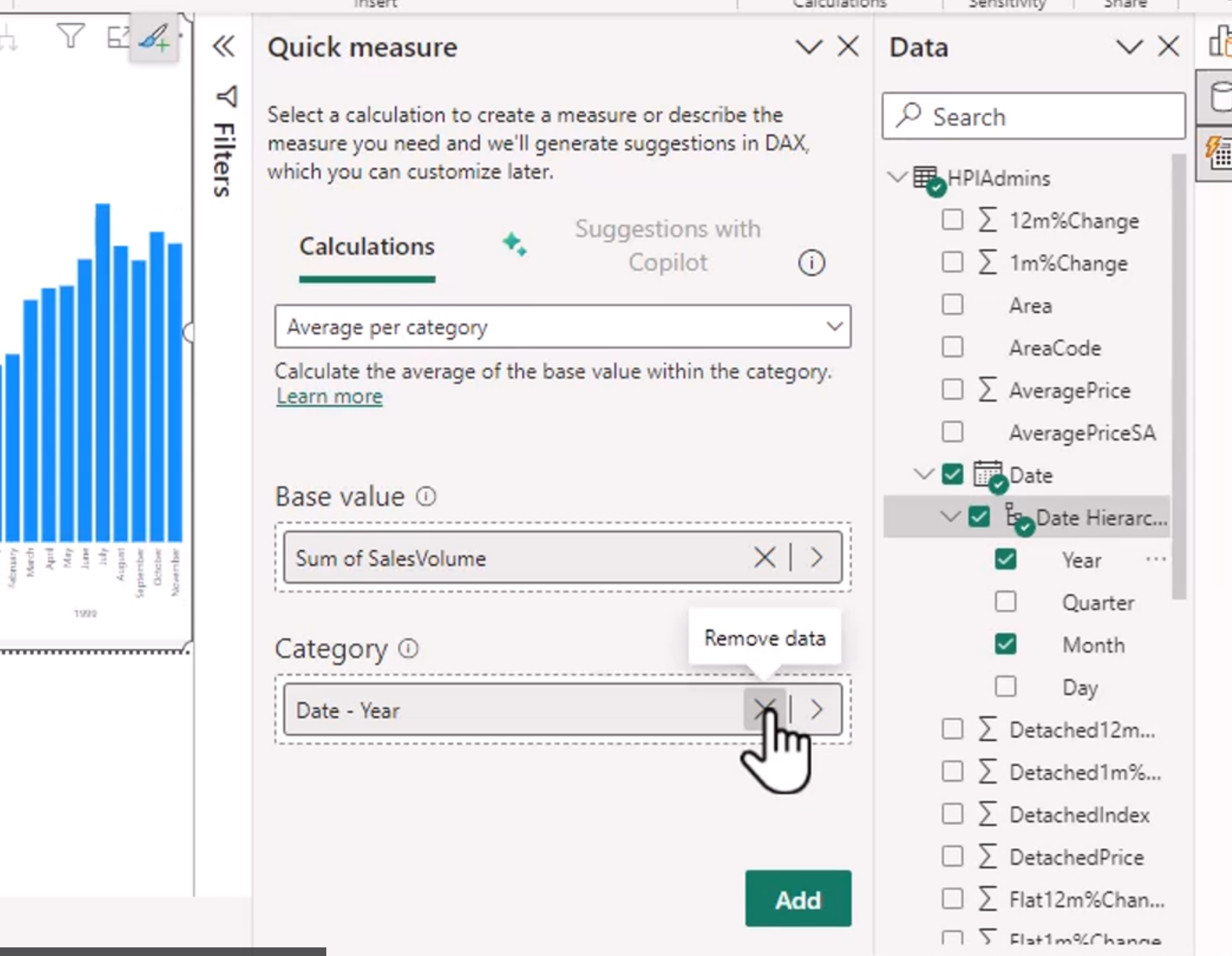
This interface is especially useful when you are learning the patterns of DAX. You can pick a measure type, choose the fields involved, and see exactly how Power BI creates the calculation. It is a practical way to understand the structure of formulas without getting lost in the details of DAX syntax.
Adding this does this:
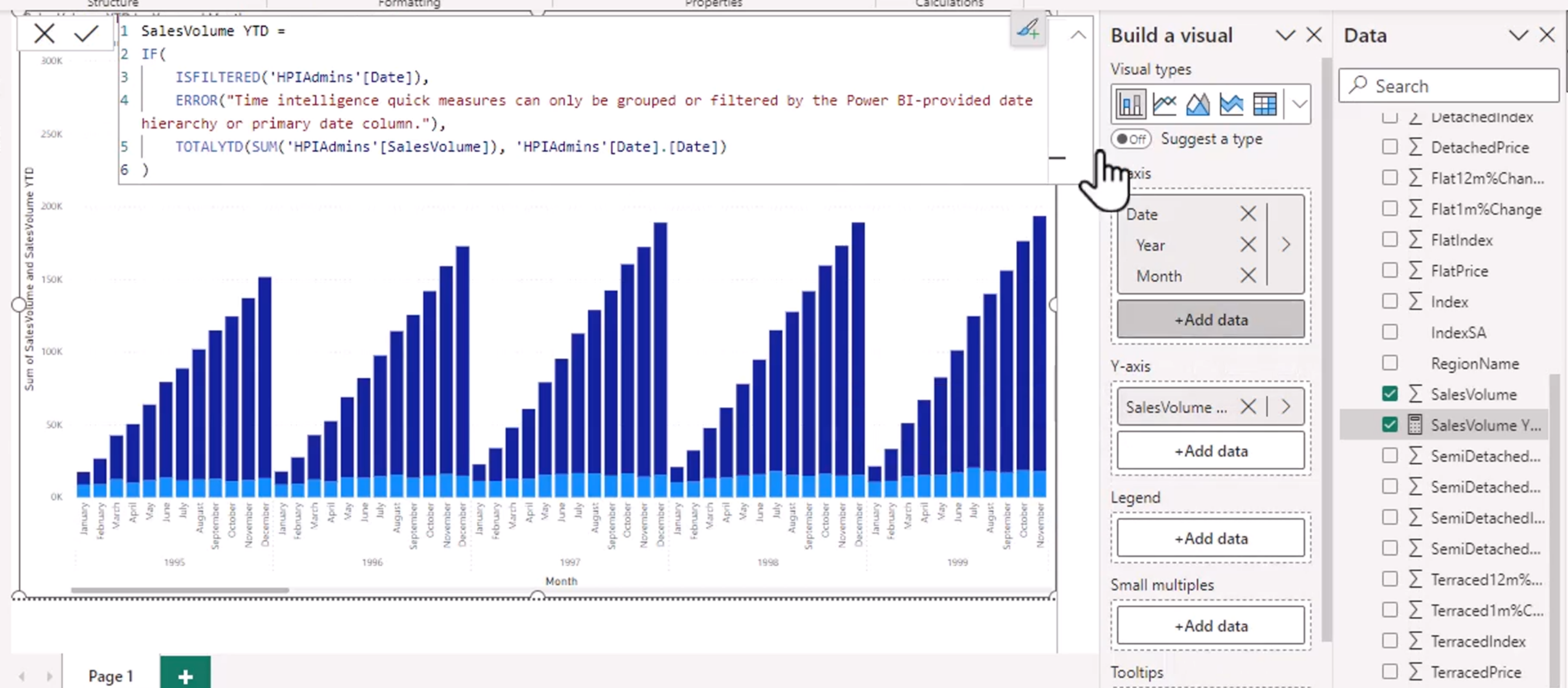
This means that once you add the quick measure, the visual responds by showing the calculated result automatically. In other words, the measure becomes part of the analysis layer and helps reveal the pattern in the visual.
A common example is a quick measure like year-over-year change or moving average. The visual may then show a trend that is easier to understand, such as growth, decline, or seasonality. This helps your audience see what is happening in the business rather than focus on the formula itself.
Quick measures are also useful because they are easy to edit and refine. Once the formula has been generated, you can inspect it in the formula bar and modify it if needed. This gives you a safer path for learning DAX: start with a generated measure, understand it, then customize it to meet your exact requirement.
There are some important things to keep in mind:
- Quick measures are best for standard, common calculations.
- They are ideal for exploration and for learning DAX patterns.
- They may not be the best choice for highly customized logic.
- Once you understand the pattern, it can be more efficient to write the DAX yourself for greater control.
This is the key balance: quick measures are fast and approachable, while custom DAX gives you more precision and flexibility.
For example, a quick measure might calculate Total Sales as the sum of a sales amount column. That is perfectly good for a dashboard. But if you need a more specific formula involving multiple conditions, time intelligence logic, or custom filters, it may be better to write the DAX explicitly.
The real value of quick measures is that they reduce friction. They let you test hypotheses quickly, create useful calculations early, and iterate rapidly while designing a report. That is exactly what makes them so helpful in a business intelligence workflow.
In practice, quick measures are often used in the early stages of a report to answer urgent analytical questions. Once the report is proven useful, you can revisit the formulas and decide whether to keep the generated version or replace it with custom DAX for better readability, performance, or maintainability.
As your Power BI skills grow, you will likely use quick measures less as a final solution and more as a learning and productivity tool. But even experienced users still rely on them for rapid prototyping and for reviewing common calculation patterns they do not want to rewrite manually every time.
So the idea is simple: quick measures help you turn raw data into meaningful insight quickly, while also acting as a practical way to learn how the DAX logic behind the scenes is built.
Export Report Data
Exporting data from Power BI Desktop is a practical way to take the results of your analysis out of the report and into a file that can be reviewed, edited, or shared elsewhere. This is especially useful when you want to move beyond the visual itself and work with the actual numbers behind it. Unlike a screenshot, an exported dataset gives you the underlying information that supports the chart, table, or KPI you have built.
This is different from the web version because Power BI Desktop is the environment where the report is being created and tested. In Desktop, you are working with the actual model, current filters, and visual context, which means the data you export is usually a direct reflection of what the report is showing at the moment. That makes it a powerful tool for validation, troubleshooting, and handoff work.
The export process is typically done from a visual. In a table or matrix visual, you can often right-click the visual and choose Export data. Power BI will then export the rows and values that are visible in that visual, based on the filters and summarization currently applied. In a chart, the export may include the underlying data used to build the chart rather than just the rendered image, depending on the type of visual and the data model.
This is helpful in situations where you need to:
- verify that the numbers in a visual match the business expectation
- send filtered results to a colleague in Excel
- review the raw values behind a chart before publishing
- confirm that a measure, slicer, or filter is working correctly
- create a quick spreadsheet for further analysis outside Power BI
One of the main benefits of exporting from Power BI Desktop is that it helps with debugging. If a visual appears incorrect or a calculation seems off, exporting the data allows you to inspect the exact rows and values being used. This is often faster than trying to infer the issue from the visual alone.
There are also a few important limitations to keep in mind. Export is usually most useful for summarized or filtered results, not always for every underlying row in a large model. Some visuals do not support full data export, and some data may be aggregated before it is exported. If the dataset is huge, the exported file might be a subset of the data rather than a complete raw table. This is especially important to remember when you are working with highly summarized visuals or hierarchical data.
Another key consideration is that Power BI exports the data that is visible in the report context, which means the output respects the current filters, slicers, and aggregations. That makes the exported file a great way to validate the report logic. If your filter is set to a specific year, product, or region, the exported output should reflect that selected context.
This is also useful when sharing with stakeholders who prefer working in Excel. An exported CSV or Excel file can be opened quickly and used for supplemental analysis, simple calculations, or a follow-up review. It is often easier for someone to open a spreadsheet and inspect the numbers than to interpret a visual in a dashboard without context.
The key idea is that exporting data is not about replacing the report. It is about taking the evidence behind the report and moving it into a more usable format. A visual tells the story, but the exported data gives the proof. That is why this capability is so valuable in Power BI Desktop.
In practice, export data when you need to check the detail, communicate the evidence, or move the result into another tool. It is a simple but highly useful step in the analysis workflow and an excellent way to bridge the gap between reporting and deeper review.
This is the Desktop-specific version of a common BI task: move from insight to evidence. The visual shows the outcome, and the export lets you inspect the underlying data that created it.
Quick Export Checklist
- Open the report in Power BI Desktop.
- Click on the visual that you want to inspect.
- Right-click the visual or use the visual menu.
- Choose "Export data".
- Select the file type and destination for the export.
- Review the exported results to confirm they match the visible filters and aggregations.
- Use the exported file for validation, Excel analysis, or stakeholder sharing.
This lets you move quickly from a visual insight to a reviewable data file without leaving the Desktop workflow.
Create Reference Lines
Reference lines are a powerful feature in Power BI that allow you to add context to your visuals by highlighting specific values or thresholds. They can be used to indicate targets, averages, benchmarks, or any other significant point that helps viewers interpret the data more effectively. By adding reference lines, you can make your charts more informative and easier to understand, as they provide a visual cue that draws attention to important aspects of the data.
Reference lines live in the Format pane of a visual, and they can be customized in terms of color, style, and label. You can add multiple reference lines to a single visual, each representing different metrics or thresholds. This flexibility allows you to create a richer narrative around your data.
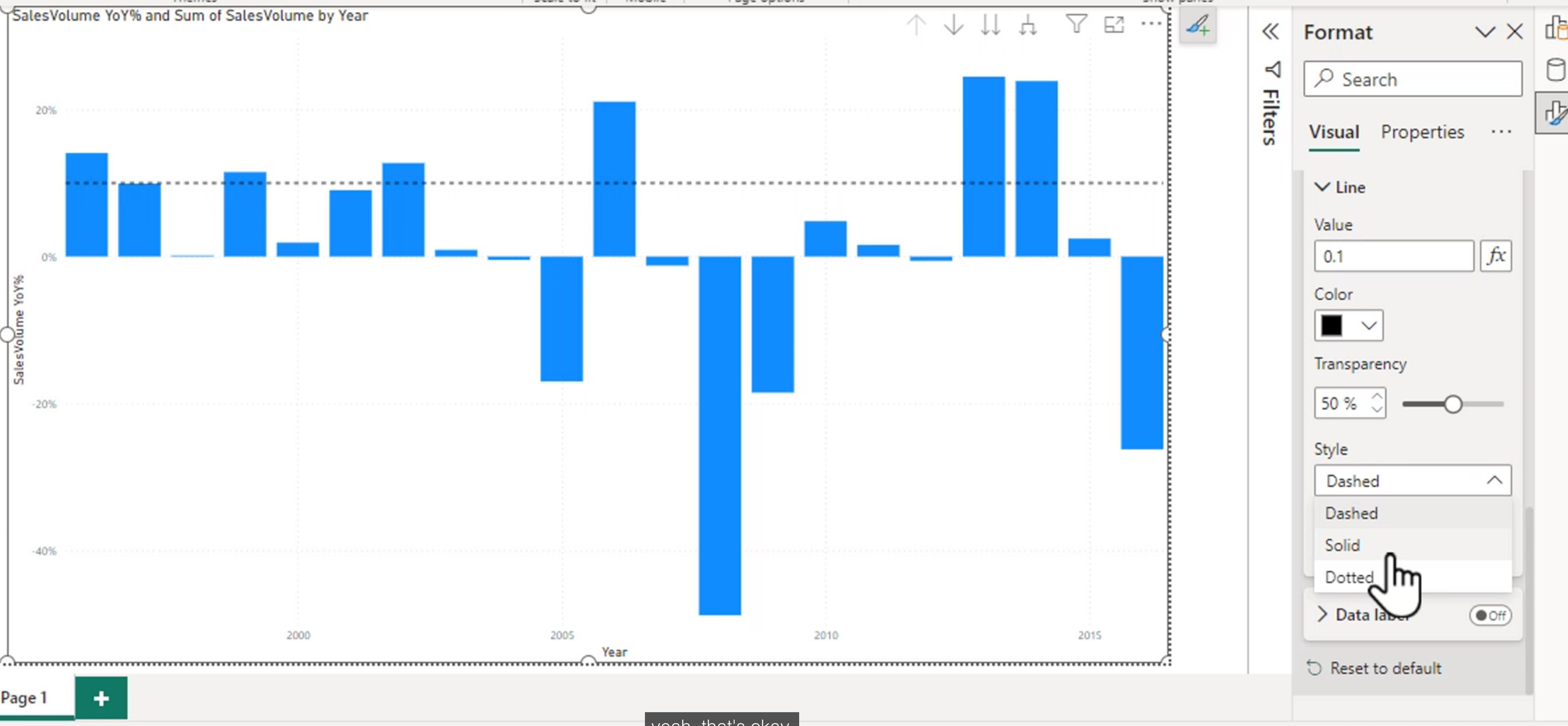
A clustered chart will have options for minimum line, maximum line, average line, and constant line. Each of these serves a different purpose:
- Minimum Line: Highlights the lowest value in the dataset, helping to identify outliers or the lower bound of performance.
- Maximum Line: Highlights the highest value, which can be useful for setting upper limits or identifying peaks in the data.
- Average Line: Displays the mean value, providing a quick reference for overall performance and helping to contextualize individual data points.
- Constant Line: Allows you to set a specific value as a reference, which can be useful for targets, thresholds, or any other fixed point of interest. You can customize the constant line to represent a specific goal or benchmark that is relevant to your analysis. This is particularly useful in business scenarios where you want to show how actual performance compares to a predefined target.
On a scatter chart, you can have a constant on both the X and Y axes. This is useful for highlighting specific thresholds or limits in two dimensions, allowing you to see how data points relate to these reference values.
These can only be used in certain charts, such as bar charts, line charts, and scatter plots. They are not available in all visual types, so it is important to check the capabilities of the specific visual you are working with. How would you even put a reference line on a pie chart? It would be meaningless, as the pie chart is not designed to show continuous data or thresholds.
Error Bars
Error bars are a visual representation of the variability or uncertainty in your data. They provide a graphical indication of the potential error or range of values around a data point, helping viewers understand the reliability and precision of the measurements being presented. In Power BI, error bars can be added to certain chart types, such as line charts and scatter plots, to give context to the data points and highlight the degree of confidence in the results.
Error bars extend above and below a plotted value. The length of the bar represents the amount of uncertainty, variation, or expected range associated with that value. They do not automatically mean that the data is statistically significant or that the range is a formal confidence interval. The meaning depends on the measure used to calculate the upper and lower bounds.
Absolute Error Bars
Absolute error uses a fixed amount in the original unit of the measure. For example, if a chart shows average delivery time and the absolute error is 2 days, a value of 10 days is displayed with a range from 8 to 12 days. A value of 30 days with the same error is displayed from 28 to 32 days.
The distance is the same for every data point:
Lower bound = Value - Absolute error
Upper bound = Value + Absolute error
Absolute error is useful when the measurement process has a consistent margin of error or when the audience understands the uncertainty in the original unit. Examples include:
- A laboratory measurement with an uncertainty of plus or minus 0.5 degrees.
- A forecast with a known error of plus or minus 100 units.
- A survey estimate where the margin of error is expressed as a fixed number of people.
In Power BI, configure the error bar to use an absolute value or measures that return the lower and upper bounds. If you use a constant error value, confirm that the same amount is meaningful across the entire chart.
Relative Error Bars
Relative error is expressed as a percentage of the plotted value. For example, if a sales value is 1,000 and the relative error is 10 percent, the range is 900 to 1,100. If the value is 10,000 with the same relative error, the range is 9,000 to 11,000.
The range changes in proportion to the value:
Lower bound = Value * (1 - Relative error)
Upper bound = Value * (1 + Relative error)
Relative error is useful when uncertainty grows with the size of the measurement. Examples include:
- A forecast expected to vary by 10 percent regardless of scale.
- Revenue estimates where larger totals naturally have larger uncertainty.
- Sensor or sampling results where precision is proportional to the measured value.
In Power BI, use a percentage-based error setting or measures that calculate the percentage bounds. Make sure the percentage is stored and formatted consistently. A value of 0.10 represents 10 percent in a calculation, while a displayed value of 10% may be stored as the same decimal value.
Choosing Between Absolute and Relative
Choose the error type based on how the uncertainty is generated:
| Situation | Suitable error type | Example |
|---|---|---|
| The same number of units may be wrong for every observation | Absolute | Plus or minus 2 days |
| The uncertainty grows with the value | Relative | Plus or minus 10 percent |
| Values have different scales but the same percentage of uncertainty | Relative | Forecasts with a 5 percent error range |
| The measurement instrument has a fixed precision | Absolute | Plus or minus 0.1 grams |
Do not choose an error type only because it makes the chart look clearer. The error range should have a defensible meaning, and the title or subtitle should explain whether it represents a margin of error, standard deviation, standard error, prediction interval, or another quantity.
Adding Error Bars in Power BI
For a supported visual:
- Select a line, column, bar, or scatter visual.
- Open the Analytics or Format pane, depending on the current Power BI interface.
- Locate Error bars and turn them on.
- Choose the series and specify the upper and lower bound method.
- Use a constant, percentage, or measure when available in the selected visual.
- Format the color, cap style, transparency, and data labels so the bars remain visible without overpowering the data.
- Add a title or subtitle that explains what the bars represent.
For a more controlled model, create measures for the bounds. A generic pattern is:
Lower Bound = [Value Measure] - [Error Measure]
Upper Bound = [Value Measure] + [Error Measure]
For a relative error of 10 percent:
Lower Bound = [Value Measure] * 0.90
Upper Bound = [Value Measure] * 1.10
The exact field wells and supported bound options vary by visual and Power BI version. If the visual does not expose error bars, use a line chart with upper and lower-bound measures, or use an error band when the visual supports it.
Interpreting Error Bars
Error bars make it easier to compare both the central value and the range around it. If two ranges overlap, that does not automatically prove that the values are the same. Likewise, non-overlapping ranges do not automatically prove statistical significance unless the ranges were calculated using an appropriate statistical method.
Use error bars to ask questions such as:
- Which values have the greatest uncertainty?
- Is the apparent difference between categories large compared with the expected variation?
- Does uncertainty increase over time or across segments?
- Are outliers still unusual after their expected range is considered?
Always verify that lower bounds are valid for the measure. A percentage calculation can produce a negative lower bound for a quantity that cannot be negative, such as a count. In that case, use a suitable lower limit or a calculation that reflects the distribution of the data.
Error Band
An error band is a shaded area around a line or curve in a chart that represents the range of uncertainty or variability in the data. It provides a visual indication of how much the data points may deviate from the expected value, helping viewers understand the potential error or confidence interval associated with the measurements. Error bands are particularly useful in line charts and scatter plots, where they can illustrate the degree of confidence in trends or predictions.
The blue area here represents the space between the lower and upper bounds:
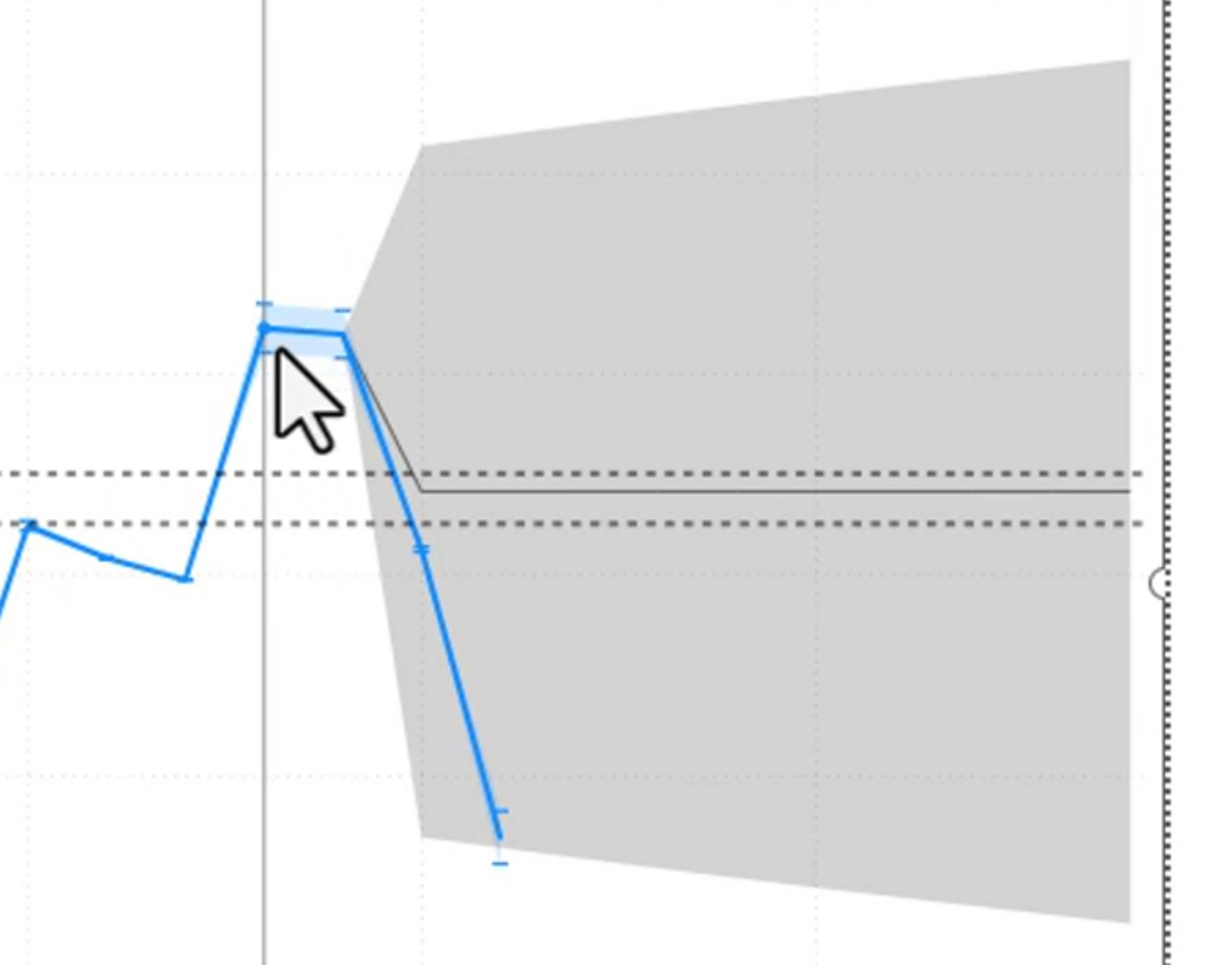
An error band is especially useful for a time series because it shows how uncertainty changes along with the trend. A narrow band suggests a more precise estimate, while a wide band indicates greater variability or uncertainty. The band should be based on a meaningful calculation, such as a forecast interval, standard deviation range, or confidence interval.
Error bars emphasize individual observations; an error band emphasizes the range around a continuous line. Use error bars when the uncertainty of separate points matters most, and use an error band when the story is about the uncertainty of a trend.
When building an error-band visual, keep the central line visually stronger than the band. Use transparency so the underlying data remains visible, include a legend or subtitle explaining the band, and avoid implying that the band is a confidence interval unless it was calculated as one.
A Practical Pattern-Finding Workflow
When identifying patterns, start with a clear business question and then choose the feature that best answers it:
- Describe the result with a card, table, or chart.
- Compare the result with a target, benchmark, or previous period.
- Investigate variation with error bars or an error band when uncertainty matters.
- Validate the detail by exporting the visual data and checking filters and calculations.
- Explain the result with a clear title, subtitle, and supporting narrative.
This sequence separates observation from interpretation. A visual may show that sales dropped, but a comparison or additional breakdown is needed before claiming why the drop occurred.
Choosing the Right Feature
| Question | Useful Power BI feature |
|---|---|
| What is the current value? | Card or multirow card |
| Are we meeting a goal? | KPI, gauge, or constant line |
| How does performance compare with a benchmark? | Reference line |
| How much variation surrounds the value? | Error bars or error band |
| What data produced this visual? | Export data |
| How can I prototype a calculation? | Quick measure |
Use the feature to support the question rather than decorate the page. A gauge is useful for progress toward a single target, while a line chart is usually better for showing a target over time.
Module 11 Summary
Module 11 introduces tools that move a report from displaying values to explaining performance:
- Quick measures generate common DAX patterns and support exploration.
- Exported data helps validate the values behind a visual.
- Reference lines add targets, averages, and thresholds to supported charts.
- Absolute error bars use a fixed amount, while relative error bars use a percentage.
- Error bands show uncertainty or variation continuously around a line.
- Labels and formatting should explain what a benchmark or uncertainty range represents.